2018 Midterms results by county

Another post related to US elections and mapping! After my previous analysis of the 2016 presidential elections, it just makes sense to come back to this topic after the recent midterms. Public availability of election data has not improved greatly since the last time I checked, but luckily I was able to conveniently get all (well, most) results from the New York Times results page, without any time-consuming scraping. How so? The data for the interactive visualization is pulled from a publicly accessible JSON file!

As always, you can follow along with the Jupyter notebook on my Github. In my previous analysis, I was a beginner with (geo)pandas and for the most part extracted all data into separate variables to work with. This time, I made a point to try to follow best practices and work within Dataframes.

Data

The data used here comes from the NYT and the US Census website. In particular, we have:

• The aforementioned JSON file, which contains results for all races (US house, US senate, state governors, propositions) that took place on November 11, 2016. I focused on US house races for the most part.

  Results were missing for a handful of races, where the incumbent candidate was uncontested and therefore won by default. For most of those, I was able to get the updated (obviously lopsided) vote counts from Ballotpedia.org. At the end, no results could be found anywhere for four Florida races: even the official Florida election page is not updated.

• From the US Census bureau, I downloaded shapefiles for 116th Congress districts, state and counties boundaries, as well as county-level population estimates

I am making available the combined data in the GeoJSON format on my GitHub, see below.

Results

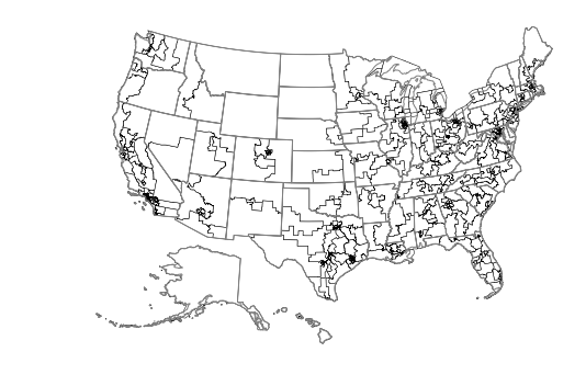
Working with the data was relatively straightforward. All shapefiles are easily loaded/processed with geopandas, for example, here I load the US state maps and the congressional district boundaries, and add the state 2-letter abbreviation from the former to the latter:

cd = gpd.GeoDataFrame.from_file(os.path.join(os.path.pardir, 'input',"tl_2018_us_cd116/tl_2018_us_cd116.dbf"))

us_df = gpd.read_file(os.path.join(os.path.pardir, 'input','cb_2017_us_state_20m.shp'))

cd = pd.merge(cd, us_df[['GEOID','STUSPS']], left_on='STATEFP', right_on='GEOID', how='left')

One of the common issues with mapping the United States is deciding where to put Alaska and Hawaii. My solution is the following:

• for Hawaii, I filter out the many small islands that trail to the West of the main archipelago (the cutoff I took is -161 degree of longitude, somehwat arbitrarily chosen) with shapely.ops.transform. I then shift the coordinates with shapely.affinity.translate to lay below Texas.
• for Alaska, first I mod the longitude (because certain Aleutian islands pass through the -180 meridian), and then with shapely.affinity.affine_transform I rescale down and translate the boundaries (downscaling is by a little over half, otherwise Alaska would be huge compared to the rest of the states). The parameters of the rescaling were taken somewhat randomly until it looked ok.

def filter_HI(x, y):
    """Only keep main Hawaii islands, drop tail far west"""
    return zip(*filter(lambda x: x[0]> -161, zip(x,y)))
def mod_long(x, y, z=None):
    """Some Aleutian archipelago islands cross the -180 longitude point. Mod longitude to bring them close to the rest."""
    return (np.mod(x,-360), y)

rest = cd[~cd['STUSPS'].isin(['HI','AK'])]

temp = cd[cd['STUSPS'].isin(['HI'])].copy()
temp.geometry = temp.geometry.apply(lambda x: shapely.ops.transform(filter_HI, x))
temp.geometry = temp.geometry.apply(lambda x: shapely.affinity.translate(x, xoff=57, yoff=3))
tempHI = temp.copy()

temp = cd[cd['STUSPS'].isin(['AK'])].copy()
temp.geometry = temp.geometry.apply(lambda x: shapely.ops.transform(mod_long, x))
temp.geometry = temp.geometry.apply(lambda x: shapely.affinity.affine_transform(x, matrix=[0.3,0,0,0.44,-65,-1]))

cd_shifted = gpd.GeoDataFrame(pd.concat([rest, tempHI, temp], ignore_index=True), crs=rest.crs).to_crs(epsg=2163)

Loading the data from the JSON file is also simple: first we dump the contents into a dictionary, which is then parsed for the relevant information, which goes into a dictionary cd_votes.

with open(os.path.join(os.path.pardir, 'input',"usa_midterms_2018-11-06.json")) as json_data:
    data = json.load(json_data)

cd_votes = defaultdict(dict)
for row in data['races']:
    if row['office'] != 'U.S. House':
        continue

    cd116fp = '00' if 'large' in row['seat_name'].lower() else "{:02d}".format(row['seat'])
    state = row['state_id']
    fips = state + cd116fp
    for c in row['candidates']:
        cd_votes[fips][c['party_id']] = c['votes']

The keys for the cd_votes dictionary are in the STXX format, where ST is the 2-letter state abbreviation and XX is the house district number. For each district, we then have per-party vote counts.

As it turns out, there are A LOT of non-mainstream parties. For simplicity, I only consider four main parties (Democrat, Republican, Green, Libertarian) and conflate all the other votes into the Independent category.

cddf = pd.DataFrame.from_dict(cd_votes, orient='index').fillna(value=0).astype(int)

keep_columns = [u'green', u'libertarian', u'republican', u'democrat']
indep = sum([cddf[c] for c in cddf.columns if c not in keep_columns])
cddf = cddf[keep_columns]
cddf['independent'] = indep
cddf['FIPS'] = cddf.index

cddf['total'] = cddf[keep_columns + [u'independent']].T.sum()
cddf['margin'] = (cddf['democrat'] - cddf['republican'])/(cddf['total']+1)

dd = pd.merge(cd_shifted, cddf, on='FIPS')
dd.plot(column='margin', cmap=cmap, figsize=(12,7.5), vmin=-1, vmax=1)
us_df.plot(ax=plt.gca(), edgecolor='w', facecolor=(0,0,0,0))

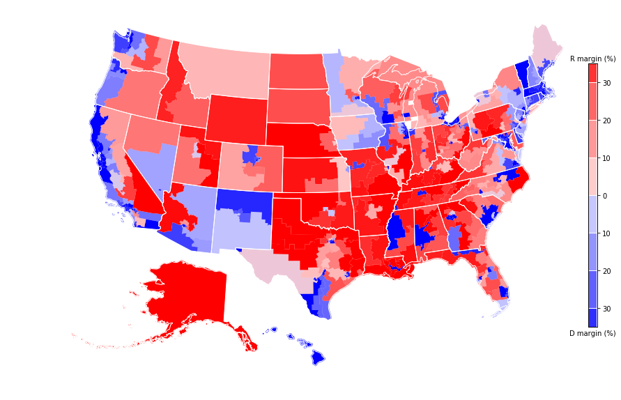
County-level maps

The map above shows congressional districts, which in most cases span multiple counties (the extreme cases are the states with only one congressional district).

It is relatively straightforward to go from district-level to county-level data: this is because the election data itself is breakdown at the county level (the JSON file has data['races'][i]['counties'] specifying how many votes each candidate received in each county that makes the district):

counties_votes = defaultdict(lambda: defaultdict(int))

for row in data['races']:
    if row['office'] != 'U.S. House':
        continue

    candidate_keys_parties = []
    for c in row['candidates']:
        candidate_keys_parties.append([c['candidate_key'], c['party_id']])

    for county in row['counties']:
        fips = county['fips']
        for c, p in candidate_keys_parties:
            counties_votes[fips][p] += county['results'][c]

df = pd.DataFrame.from_dict(counties_votes, orient='index', dtype=int).fillna(value=0).astype(int)

We have parsed the JSON file as was done previously, except now we are iterating over the counties in each district, and for each county tallying the vote by party. If a county spans multiple districts, the dictionary is first created and then more votes are added to it when it is visited by iterating over the other districts. We then create a Dataframe and (not shown in the snippet above) as before, we conflate all non-major-party votes into the Independent category.

Short aside: what to do with the uncontested races? In those cases, I could get the vote totals from Ballotpedia, but getting the county breakdown would have meant to go through each state official election results portal, and that seemed like too much work to yours truly (plus, I knew for sure of the four Florida races where no results are available at all). A crude estimate is the following: the votes can be split according to the fraction (in terms of area) of the district that each county occupies. So if a district fully covers two counties and half-covers one, the three counties will get 2/5, 2/5 and 1/5 of the total votes (in this example all counties have the same area). Obviously this is a crude estimate (for example basing it on number of voters would be better), but it’s the simplest approach given the lack of data. At the end of the day, it should not matter too much as this step is taken only for the handful of uncontested races.

Shorter aside: Alaska reports its result by precinct and not by county (or borough as they are called there), which means that not even the NYT has county-level results. Because of this, and because just splitting the votes with respect to the counties would not be accurate at all (this time this is not an uncontested race, so the margins matter), I drop Alaska from the analysis.

Now I can load the counties shapefiles, shift Alaska and Hawaii, and merge them with the county-level votes dataframe I created above. The result is the following county-level map:

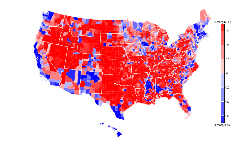
Notice how even in states with a single house district, there is a lot of internal variability (most visible in Montana, Idaho and the Dakotas).

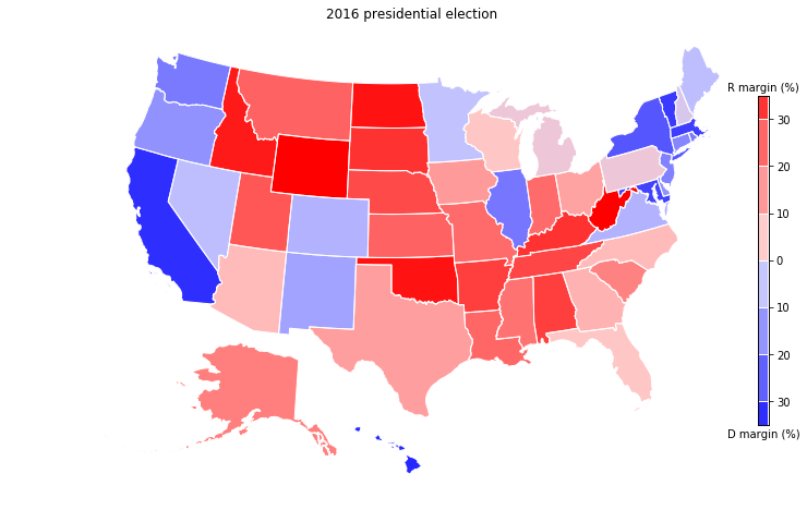
Now, because I had already created similar maps for my cartogram project, I can show the 2018 (left) and 2016 (right) maps side by side:

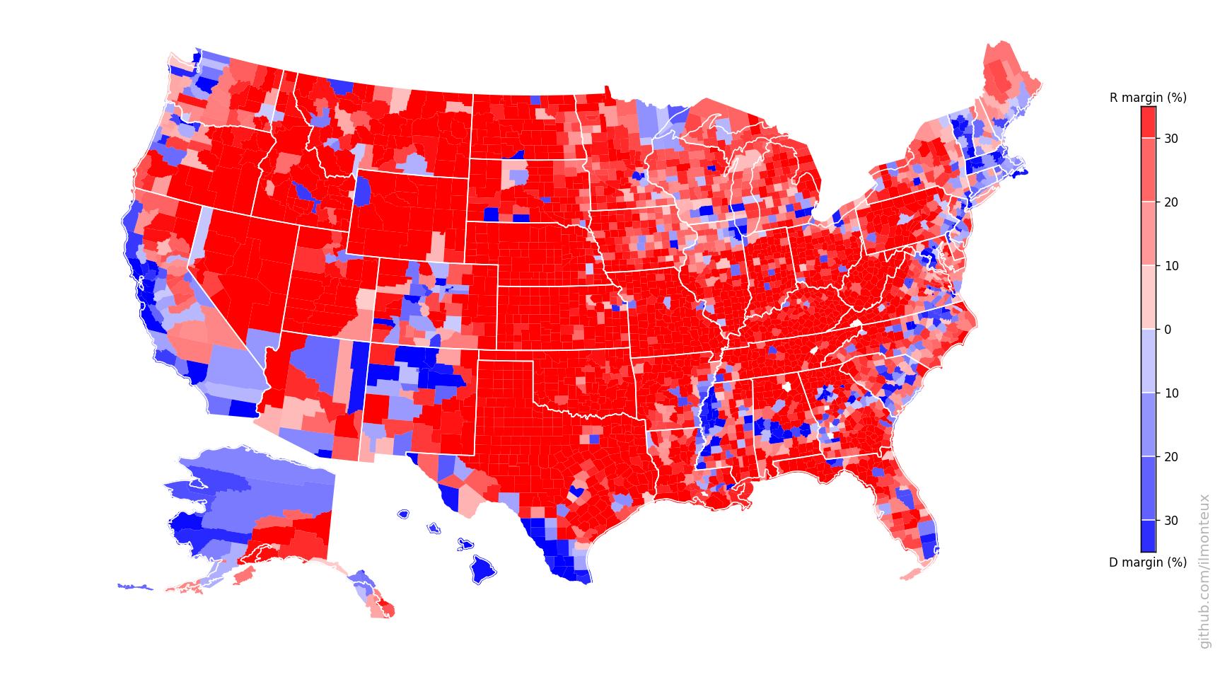
Note: technically the 2016 map was made by looking at the presidential vote, while the 2018 map shows the House vote, so the comparison should be taken with a grain of salt.

State-level results and trends

Finally, we can group the midterm election by state, and get a coarser picture. Because individual states are what decides the presidential election through the Electoral College, a comparison to the 2016 results is here more apt.

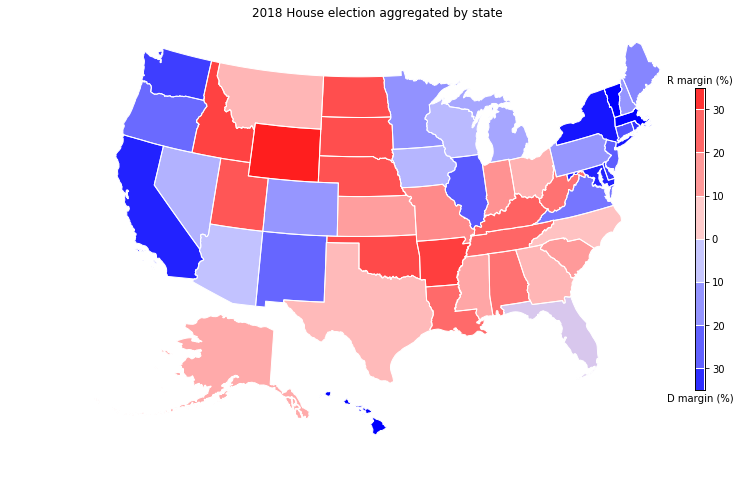
Just a quick glance shows the big differences. With New Hampshire, Pennsylvania, Michigan, Wisconsin, Iowa and Arizona turning blue, 67 electoral college votes would have flipped, electing Hillary with about the same margin Trump won.

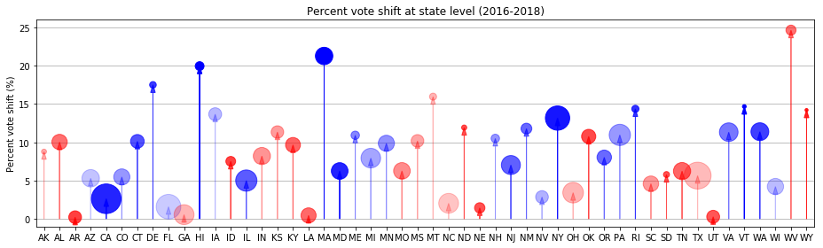
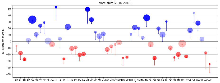
Overall, every state shifted towards Democrats (as can be expected in a wave election), some of them more than others.

Conclusions

That’s it for now! It would be fun to make cartograms of the above maps following my cartograms project, but that’s all I had time for this weekend.

The combined dataset is 220 MB and can be downloaded from my AWS account:

• Counties + votes: https://s3-us-west-2.amazonaws.com/dumpilmonteux/2018_midterms_votes_no_fill.geojson

• Counties + votes (including estimate from uncontested races): https://s3-us-west-2.amazonaws.com/dumpilmonteux/2018_midterms_votes.geojson