Metrics for semantic segmentation
In this post, I will discuss semantic segmentation, and in particular evaluation metrics useful to assess the quality of a model. Semantic segmentation is simply the act of recognizing what is in an image, that is, of differentiating (segmenting) regions based on their different meaning (semantic properties).
This post is a prelude to a semantic segmentation tutorial, where I will implement different models in Keras. While working on that, I noticed the absence of good materials online so I decided to make a separate post specifically about metrics. For a quick introduction that covers most bases, see this post and this other one by Jeremy Jordan.
Imagine you are a self-driving car going on your merry way along a road: within all the sensors that help the computer build a representation of the outside world, an essential part will be cameras. For each frame, the car will need to evaluate where the road is, any street sign or light, and finally if there are any obstacles on its way (people, bicycles, walls, other cars). This is where semantic segmentation comes in: the goal is to classify every pixel in the image as representing a certain class (e.g., person, car, street, sidewalk, speed limit, etc…).
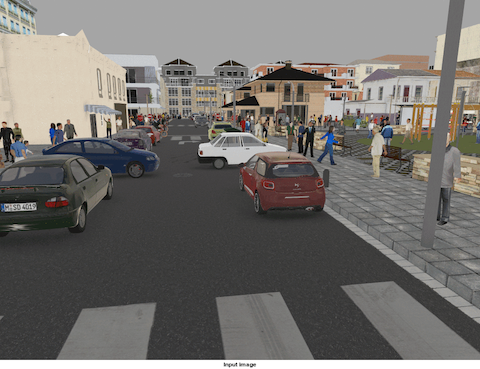
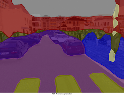
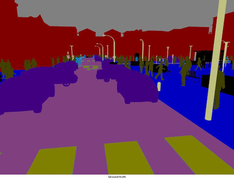
Left: input image. Center: predicted masks (FCN-8 model). Right: ground truths. Image source: NVIDIA blog
How does one measure the success of a model? In the example above, segmentation worked well for the street/sidewalk/crosswalk demarcation, as well as for cars and people, but most lamp posts were missed. In addition, the model correctly identified people (in brown), but was terrible at pinning down their exact locations. Even for the good predictions, one can see that the predicted objects overflow around the true objects. Well-defined metrics will help us grade models.
Metrics
Intuitively, a successful prediction is one which maximizes the overlap between the predicted and true objects. Two related but different metrics for this goal are the Dice and Jaccard coefficients (or indices):
Here, and are two segmentation masks for a given class (but the formulas are general, that is, you could calculate this for anything, e.g. a circle and a square), is the norm of (for images, the area in pixels), and , are the intersection and union operators.
Both the Dice and Jaccard indices are bounded between 0 (when there is no overlap) and 1 (when A and B match perfectly). The Jaccard index is also known as Intersection over Union (IoU) and because of its simple and intuitive expression is widely used in computer vision applications.
In terms of the confusion matrix, the metrics can be rephrased in terms of true/false positives/negatives:
Here is an illustration of the Dice and IoU metrics given two circles representing the ground truth and the predicted masks for an arbitrary object class:
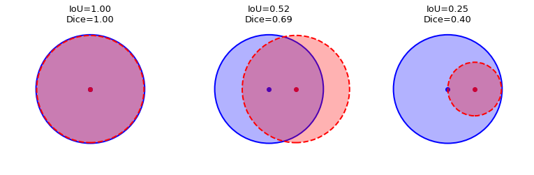
Why choose one over the other? See this StackOverflow question for a comparison between Dice and IoU. In general, the IoU is more intuitive and more commonly used.
So far, my discussion has been somewhat general. What is a segmentation mask anyway, and what does it mean to work with different classes? And how do we calculate metrics once we have our model predictions?
Let’s say that we start with a -sized image, in which we want to recognize classes of objects. Then, the output of a segmentation model will be a tensor of real numbers, that is, masks for the original image, which predict the probability of each pixel representing a certain object class (technically, the numbers are the softmax output of the model and do not necessarily correspond to a probability - we can just say it’s the model prediction). For example, in the images above, the classes are [road, car, person, lamp post, …]. If a given pixel has values [0.1, 0.2, 0.6, 0.01, …] (remember that a softmax output sums up to 1), the model’s best guess is that the pixel is part of a person (and the second best guess is that it’s a car). In most cases, we only keep the model’s best prediction, that is, we assign that pixel to the class corresponding to the max value: in this example, that pixel is assigned to the class “person” and the mask is one-hot encoded as [0, 0, 1, 0, …].
For each class, we can compute the metrics above by finding the intersection between the ground truth and predicted one-hot encoded masks for each class. Metrics can be examined class-by-class, or by taking the average over all the classes, to get a mean IoU.
Let’s simplify the discussion by looking at the following example:
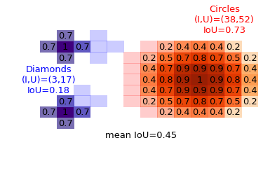
With orange and purple gradients we show the predicted masks for two object classes (with numerical values for the predictions annotated for each pixel): “circles” and “diamonds” (the class names will make more sense further down with more pixels in the images). The light red and blue pixels are the ground-truth masks for each object: for the “circle” class, the predicted and true masks are just one pixel away from each other. For the “diamond” class (at low resolution, it is more like a cross), one instance is off by two pixels horizontally while the other is one pixel away along the diagonal. The intersection and union can be found by counting pixels, with the resulting IoU metric shown above (per-class, and average).
My implementations in Numpy and Keras are shared in their own GitHub gist, but for discussion purposes I will copy the salient Numpy snippets as we go along. All images in this post have been generated in the corresponding Jupyter notebook.
# one hot encoding of predictions
num_classes = y_pred.shape[-1]
y_pred = np.array([ np.argmax(y_pred, axis=-1)==i for i in range(num_classes) ]).transpose(1,2,3,0)

axes = (1,2) # W,H axes of each image
intersection = np.sum(np.logical_and(y_pred, y_true), axis=axes)
# intersection = np.sum(np.abs(y_pred * y_true), axis=axes)
union = np.sum(np.logical_or(y_pred, y_true), axis=axes)
mask_sum = np.sum(np.abs(y_true), axis=axes) + np.sum(np.abs(y_pred), axis=axes)
# union = mask_sum  - intersection

smooth = .001
iou = (intersection + smooth) / (union + smooth)
dice = 2 * (intersection + smooth)/(mask_sum + smooth)

iou = np.mean(iou)
dice = np.mean(dice)
One can see that the implementations of IoU and Dice are almost the same, so I will only be going through the IoU computation step by step. First, we one-hot encode the predicted classes by taking the argmax function (no pixel can be predicted as being from multiple classes). Then, we take the intersection with np.logical_and() and the union with np.logical_or(), after which we sum the number of pixels in either the intersection or union. Finally, to deal with cases where classes were not present in the ground truth masks and were not predicted anywhere (which would result in intersection/union = 0/0 = nan), we add a small smoothing factor of 0.001 (note that the unit of measure here is a pixel, so 0.001 would not appreciably change results for any case with intersection or union bigger than zero) such that the IoU is 1 for those classes. We then take the mean (over the batch and class axes) to yield one number for our metric.
You can see two commented lines above showing different implementations of the intersection and union: because the masks are one-hot encoded, taking the element-wise multiplication (y_pred * y_true) is the same as doing np.logical_and(y_pred, y_true) (because 0 & 1 = 0 = 0 * 1 ). The second commented line is just an alternative computation of the union from the sum and the intersection (because ).
Soft vs hard metrics
In the above implementation, I have taken the max of the model prediction over the classes (one-hot encoding), which corresponds to drop information about everything apart from the model’s best guess. It can be argued that there is value in producing the wrong prediction if the model’s second choice would have been the correct choice. The model is still wrong, but it was almost right! Should that be reflected in the metric?
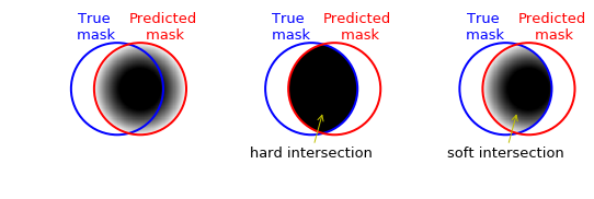
To take in account this scenario, one can define soft versions of the above metrics. For example, let’s assume that the model confidence varies within the full red circle above, such that it is highest at the center and then falls off continuously as it approaches the borders. The situation is exemplified below, with the gray shading standing for the model prediction confidence in the left plot. At the center, I use the np.logical_and(y_true, y_pred), which still works because 1 & 0.1 = 1, 1 & 0 = 0. On the right, I am simply element-wise multiplying the two masks (y_true * y_pred) which defines the soft approach (because y_true is zero everywhere except inside the blue circle, and one inside of it, multiplying y_pred by it just means zeroing out anything outside of the blue circle).
Similarly, the norm of the model output will not simply be equal to the area in pixels, but it will be weighted by the model output (in numpy, we have |A| = np.sum(A)).
We can now compare the “standard” IoU versus the soft IoU (similar results hold for the Dice coefficient). We take similar examples as in the blue-red example above, but this time the model prediction confidence varies inside the circle (the contours show the model prediction between 0 and 1).
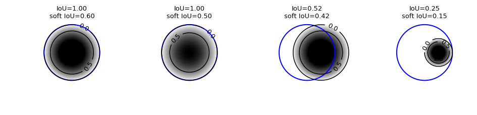
On the two left plots, we have predictions that on the geometric side match perfectly with the truth mask, but with lower confidence as one moves away from the center (the leftmost plot shows higher confidence on a larger region, while the second shows weaker confidence). In general, the soft IoU scores are generically lower than the “hard” scores, easily by a factor of 2 or more (as expected given the lower confidence as one approaches the border of the predicted object). In the center-right plot, we show a case in which the geometric positioning of the predicted circle is not perfect, but the overlap covers the highest confidence region: because of that, the soft IoU score drops only 20% from the standard version. Finally, the rightmost shows a case already seen above, with a much smaller predicted object area: as in the leftmost plot, the soft IoU is 60% of its standard value.
The differences between soft and hard IoU scores shown above are only indicative as they depend on the specific spatial distributions of model prediction confidence, which were here taken as simple functions for illustration purposes.
The is even easier to code up in Numpy than the previous “hard” versions, as we do not have to one-hot encode the predictions. We simply use element-wise multiplication.
axes = (1,2) # W,H axes of each image
intersection = np.sum(np.abs(y_pred * y_true), axis=axes)
mask_sum = np.sum(np.abs(y_true), axis=axes) + np.sum(np.abs(y_pred), axis=axes)
union = mask_sum  - intersection

smooth = .001
iou = (intersection + smooth) / (union + smooth)
dice = 2 * (intersection + smooth)/(mask_sum + smooth)

iou = np.mean(iou)
dice = np.mean(dice)
Subtleties with mean metrics
In the examples above, I have always shown one class at a time. Typical real-world applications of semantic segmentation involve tens or hundreds of classes. While the code above still works great, there are subtleties involved:
-
If an object class is not present in the image and not predicted by the model, we give it an IoU score of 1. In applications with large numbers of possible classes but only a few different objects in the same frame at the same time, this would heavily weight and raise the mean IoU: for example, with 100 possible classes and an image with only 5 of them, a naive model predicting the absence of all object classes in every picture it is fed would still achieve a mean IoU score of 0.95 (Iou=1 for 95 classes, Iou=0 for 5 classes).
-
Typically, semantic segmentation models include a background class in addition to the classes that we want to identify (e.g. people, road, cars…). The background class is a “none of the above” class, so that if we want to identify classes in an image, we actually have classes after including the background. In particular, because objects usually only take up a relatively small part of the image, even a naive model predicting background everywhere would have good metrics for the background class. When calculating metrics, we typically care more about the individual objects and not much about the background is (after all, the background class is just the complement of all the other objects, so that a good identification of the objects will translate in a good identification of the background).
-
In addition, very small objects have the potential of wildly swing the metrics given small changes in model prediction: for example, if an object only has 1 pixel in the image, models predicting 0,1,2 and 3 pixels for that class would have IoU=0,1,0.5 and 0.33.
For the second point, we can just drop the background class (usually this is the last class) before taking the mean. The last point can be fixed by requiring some minimum object size when assigning pixels to an object (anyway, we would not expect any model to be able to identify one lone pixel as an object, as there is barely any information there). For the first point, a solution is to restrict ourselves to only take the average over the classes that are present in either the true or the predicted masks. This solves the problem of counting classes that are not there, but still takes into account wanting to penalize models that predict things that are not there (in these cases, we still get IoU=0).
NB: For example, this is the Tensorflow implementation. In their case, they are being a little more careful as computing the metrics for each batch (as I am doing) can yield different results than computing the metric for the whole dataset (for example, at the end of a training epoch). See this post for a discussion of the difference.
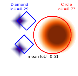
For example see the following figure, where we have two classes present (circles in red, diamonds in blue), with respective IoU’s equal to 0.73 and 0.29. The mean IoU for those classes is therefore the average, 0.51. Now, if I had been trying to segment additional classes (say two more, a square and a star) but the model had correctly identified that they are not in the image, the IoU for those absent classes would have been 1, and the mean taking all four classes would have been higher (0.75), which would be misleading.
This more advanced mean IoU computation is almost the same as above, except that we mask out the classes that do not appear. So we define a mask (a batch_size * num_classes-shaped matrix) which is zero when the class is not present and not predicted.
mask = np.not_equal(union, 0)
With this mask, we can just zero out the elements of the IoU matrix before computing the mean, by taking the element-wise multiplication iou * mask. We then have to be careful about not taking the average over those masked elements.
Numpy implementation
The full code for the Dice and IoU metrics in Numpy is below. Because the steps are almost the same for the two metrics and for taking the hard or soft metrics, I define a single function with arguments that decide which specific version of the metric should be called.
def metrics_np(y_true, y_pred, metric_name,
    metric_type='standard', drop_last = True, mean_per_class=False, verbose=False):
    """
    Compute mean metrics of two segmentation masks, via numpy.

    IoU(A,B) = |A & B| / (| A U B|)
    Dice(A,B) = 2*|A & B| / (|A| + |B|)

    Args:
        y_true: true masks, one-hot encoded.
        y_pred: predicted masks, either softmax outputs, or one-hot encoded.
        metric_name: metric to be computed, either 'iou' or 'dice'.
        metric_type: one of 'standard' (default), 'soft', 'naive'.
          In the standard version, y_pred is one-hot encoded and the mean
          is taken only over classes that are present (in y_true or y_pred).
          The 'soft' version of the metrics are computed without one-hot
          encoding y_pred.
          The 'naive' version return mean metrics where absent classes contribute
          to the class mean as 1.0 (instead of being dropped from the mean).
        drop_last = True: boolean flag to drop last class (usually reserved
          for background class in semantic segmentation)
        mean_per_class = False: return mean along batch axis for each class.
        verbose = False: print intermediate results such as intersection, union
          (as number of pixels).
    Returns:
        IoU/Dice of y_true and y_pred, as a float, unless mean_per_class == True
          in which case it returns the per-class metric, averaged over the batch.

    Inputs are B*W*H*N tensors, with
        B = batch size,
        W = width,
        H = height,
        N = number of classes
    """

    assert y_true.shape == y_pred.shape, 'Input masks should be same shape, instead are {}, {}'.format(y_true.shape, y_pred.shape)
    assert len(y_pred.shape) == 4, 'Inputs should be B*W*H*N tensors, instead have shape {}'.format(y_pred.shape)

    flag_soft = (metric_type == 'soft')
    flag_naive_mean = (metric_type == 'naive')

    num_classes = y_pred.shape[-1]
    # if only 1 class, there is no background class and it should never be dropped
    drop_last = drop_last and num_classes>1

    if not flag_soft:
        if num_classes>1:
            # get one-hot encoded masks from y_pred (true masks should already be in correct format, do it anyway)
            y_pred = np.array([ np.argmax(y_pred, axis=-1)==i for i in range(num_classes) ]).transpose(1,2,3,0)
            y_true = np.array([ np.argmax(y_true, axis=-1)==i for i in range(num_classes) ]).transpose(1,2,3,0)
        else:
            y_pred = (y_pred > 0).astype(int)
            y_true = (y_true > 0).astype(int)

    # intersection and union shapes are batch_size * n_classes (values = area in pixels)
    axes = (1,2) # W,H axes of each image
    intersection = np.sum(np.abs(y_pred * y_true), axis=axes) # or, np.logical_and(y_pred, y_true) for one-hot
    mask_sum = np.sum(np.abs(y_true), axis=axes) + np.sum(np.abs(y_pred), axis=axes)
    union = mask_sum  - intersection # or, np.logical_or(y_pred, y_true) for one-hot

    if verbose:
        print('intersection (pred*true), intersection (pred&true), union (pred+true-inters), union (pred|true)')
        print(intersection, np.sum(np.logical_and(y_pred, y_true), axis=axes), union, np.sum(np.logical_or(y_pred, y_true), axis=axes))

    smooth = .001
    iou = (intersection + smooth) / (union + smooth)
    dice = 2*(intersection + smooth)/(mask_sum + smooth)

    metric = {'iou': iou, 'dice': dice}[metric_name]

    # define mask to be 0 when no pixels are present in either y_true or y_pred, 1 otherwise
    mask =  np.not_equal(union, 0).astype(int)
    # mask = 1 - np.equal(union, 0).astype(int) # True = 1

    if drop_last:
        metric = metric[:,:-1]
        mask = mask[:,:-1]

    # return mean metrics: remaining axes are (batch, classes)
    # if mean_per_class, average over batch axis only
    # if flag_naive_mean, average over absent classes too
    if mean_per_class:
        if flag_naive_mean:
            return np.mean(metric, axis=0)
        else:
            # mean only over non-absent classes in batch (still return 1 if class absent for whole batch)
            return (np.sum(metric * mask, axis=0) + smooth)/(np.sum(mask, axis=0) + smooth)
    else:
        if flag_naive_mean:
            return np.mean(metric)
        else:
            # mean only over non-absent classes
            class_count = np.sum(mask, axis=0)
            return np.mean(np.sum(metric * mask, axis=0)[class_count!=0]/(class_count[class_count!=0]))

def mean_iou_np(y_true, y_pred, **kwargs):
    """
    Compute mean Intersection over Union of two segmentation masks, via numpy.

    Calls metrics_np(y_true, y_pred, metric_name='iou'), see there for allowed kwargs.
    """
    return metrics_np(y_true, y_pred, metric_name='iou', **kwargs)

def mean_dice_np(y_true, y_pred, **kwargs):
    """
    Compute mean Dice coefficient of two segmentation masks, via numpy.

    Calls metrics_np(y_true, y_pred, metric_name='dice'), see there for allowed kwargs.
    """
    return metrics_np(y_true, y_pred, metric_name='dice', **kwargs)
Keras implementations
The metrics translate into Keras in a straightforward way. Given how Keras (with Tensorflow backend) works, one has to replace numpy calls with corresponding calls in keras.backend or tensorflow to build the computational graph, which will be executed at computation time.
def seg_metrics(y_true, y_pred, metric_name,
    metric_type='standard', drop_last = True, mean_per_class=False, verbose=False):
    """
    Compute mean metrics of two segmentation masks, via Keras.

    IoU(A,B) = |A & B| / (| A U B|)
    Dice(A,B) = 2*|A & B| / (|A| + |B|)

    Args:
        y_true: true masks, one-hot encoded.
        y_pred: predicted masks, either softmax outputs, or one-hot encoded.
        metric_name: metric to be computed, either 'iou' or 'dice'.
        metric_type: one of 'standard' (default), 'soft', 'naive'.
          In the standard version, y_pred is one-hot encoded and the mean
          is taken only over classes that are present (in y_true or y_pred).
          The 'soft' version of the metrics are computed without one-hot
          encoding y_pred.
          The 'naive' version return mean metrics where absent classes contribute
          to the class mean as 1.0 (instead of being dropped from the mean).
        drop_last = True: boolean flag to drop last class (usually reserved
          for background class in semantic segmentation)
        mean_per_class = False: return mean along batch axis for each class.
        verbose = False: print intermediate results such as intersection, union
          (as number of pixels).
    Returns:
        IoU/Dice of y_true and y_pred, as a float, unless mean_per_class == True
          in which case it returns the per-class metric, averaged over the batch.

    Inputs are B*W*H*N tensors, with
        B = batch size,
        W = width,
        H = height,
        N = number of classes
    """

    flag_soft = (metric_type == 'soft')
    flag_naive_mean = (metric_type == 'naive')

    # always assume one or more classes
    num_classes = K.shape(y_true)[-1]

    if not flag_soft:
        # get one-hot encoded masks from y_pred (true masks should already be one-hot)
        y_pred = K.one_hot(K.argmax(y_pred), num_classes)
        y_true = K.one_hot(K.argmax(y_true), num_classes)

    # if already one-hot, could have skipped above command
    # keras uses float32 instead of float64, would give error down (but numpy arrays or keras.to_categorical gives float64)
    y_true = K.cast(y_true, 'float32')
    y_pred = K.cast(y_pred, 'float32')

    # intersection and union shapes are batch_size * n_classes (values = area in pixels)
    axes = (1,2) # W,H axes of each image
    intersection = K.sum(K.abs(y_true * y_pred), axis=axes)
    mask_sum = K.sum(K.abs(y_true), axis=axes) + K.sum(K.abs(y_pred), axis=axes)
    union = mask_sum  - intersection # or, np.logical_or(y_pred, y_true) for one-hot

    smooth = .001
    iou = (intersection + smooth) / (union + smooth)
    dice = 2 * (intersection + smooth)/(mask_sum + smooth)

    metric = {'iou': iou, 'dice': dice}[metric_name]

    # define mask to be 0 when no pixels are present in either y_true or y_pred, 1 otherwise
    mask =  K.cast(K.not_equal(union, 0), 'float32')

    if drop_last:
        metric = metric[:,:-1]
        mask = mask[:,:-1]

    if verbose:
        print('intersection, union')
        print(K.eval(intersection), K.eval(union))
        print(K.eval(intersection/union))

    # return mean metrics: remaining axes are (batch, classes)
    if flag_naive_mean:
        return K.mean(metric)

    # take mean only over non-absent classes
    class_count = K.sum(mask, axis=0)
    non_zero = tf.greater(class_count, 0)
    non_zero_sum = tf.boolean_mask(K.sum(metric * mask, axis=0), non_zero)
    non_zero_count = tf.boolean_mask(class_count, non_zero)

    if verbose:
        print('Counts of inputs with class present, metrics for non-absent classes')
        print(K.eval(class_count), K.eval(non_zero_sum / non_zero_count))

    return K.mean(non_zero_sum / non_zero_count)

def mean_iou(y_true, y_pred, **kwargs):
    """
    Compute mean Intersection over Union of two segmentation masks, via Keras.

    Calls metrics_k(y_true, y_pred, metric_name='iou'), see there for allowed kwargs.
    """
    return seg_metrics(y_true, y_pred, metric_name='iou', **kwargs)

def mean_dice(y_true, y_pred, **kwargs):
    """
    Compute mean Dice coefficient of two segmentation masks, via Keras.

    Calls metrics_k(y_true, y_pred, metric_name='iou'), see there for allowed kwargs.
    """
    return seg_metrics(y_true, y_pred, metric_name='dice', **kwargs)
Compared to the numpy code, masking out absent classes is slightly different, as one cannot simply slice through array in keras as one does in numpy. The solution was using tf.boolean_mask to select elements of the N*C metric array corresponding to non-absent classes.
Conclusions
Hopefully this post was useful to understand standard semantic segmentation metrics such as Intersection over Union or the Dice coefficient, and to see how they can be implemented in Keras for use in advanced models. In case you missed it above, the python code is shared in its GitHub gist, together with the Jupyter notebook used to generate all figures in this post. Stay tuned for the next post diving into popular deep learning models for semantic segmentation!